Physical parameters of Type II-Plateau Supernovae from Pejcha & Prieto (2015, ApJ, 806, 225)
|
Physical parameters of Type II-Plateau Supernovae from Pejcha & Prieto (2015, ApJ, 806, 225) |
|
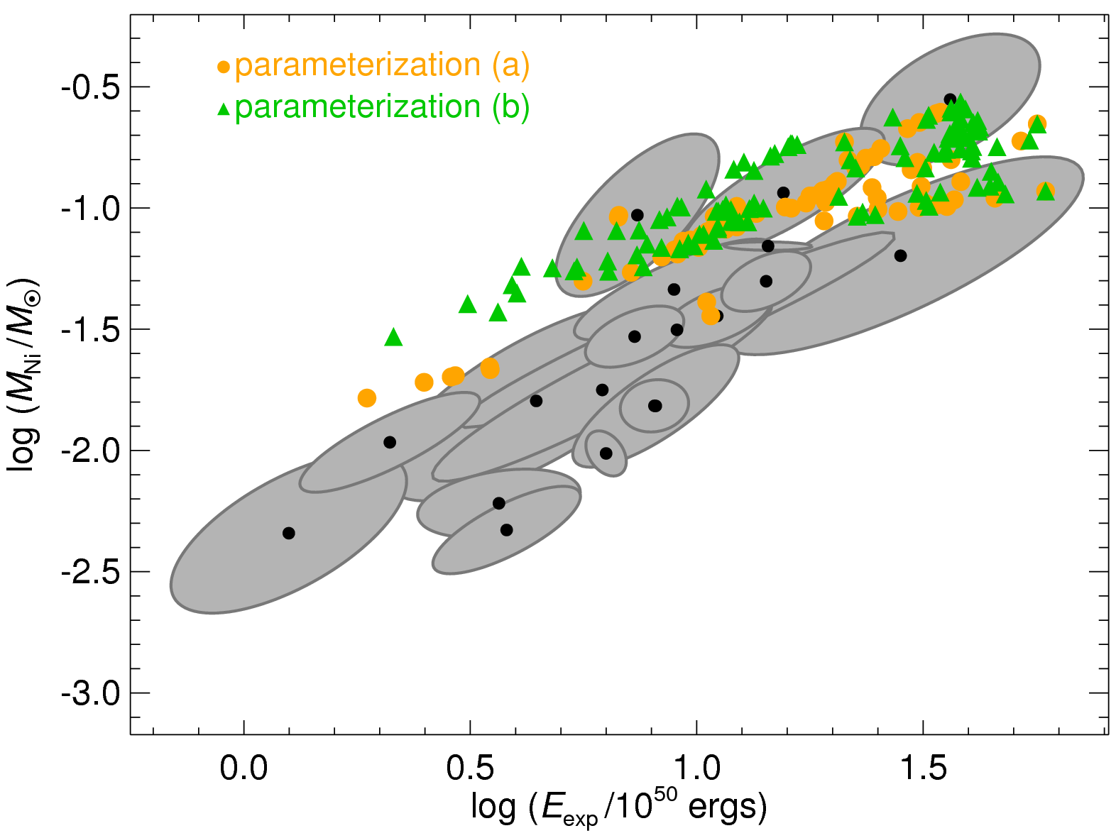 |
| Comparison of observational results from Pejcha & Prieto (2015, ApJ, 806, 225) shown with grey ellipses with the predictions of the neutrino mechanism from Pejcha & Thompson (2015, ApJ, 801, 90) shown with orange and green symbols. |
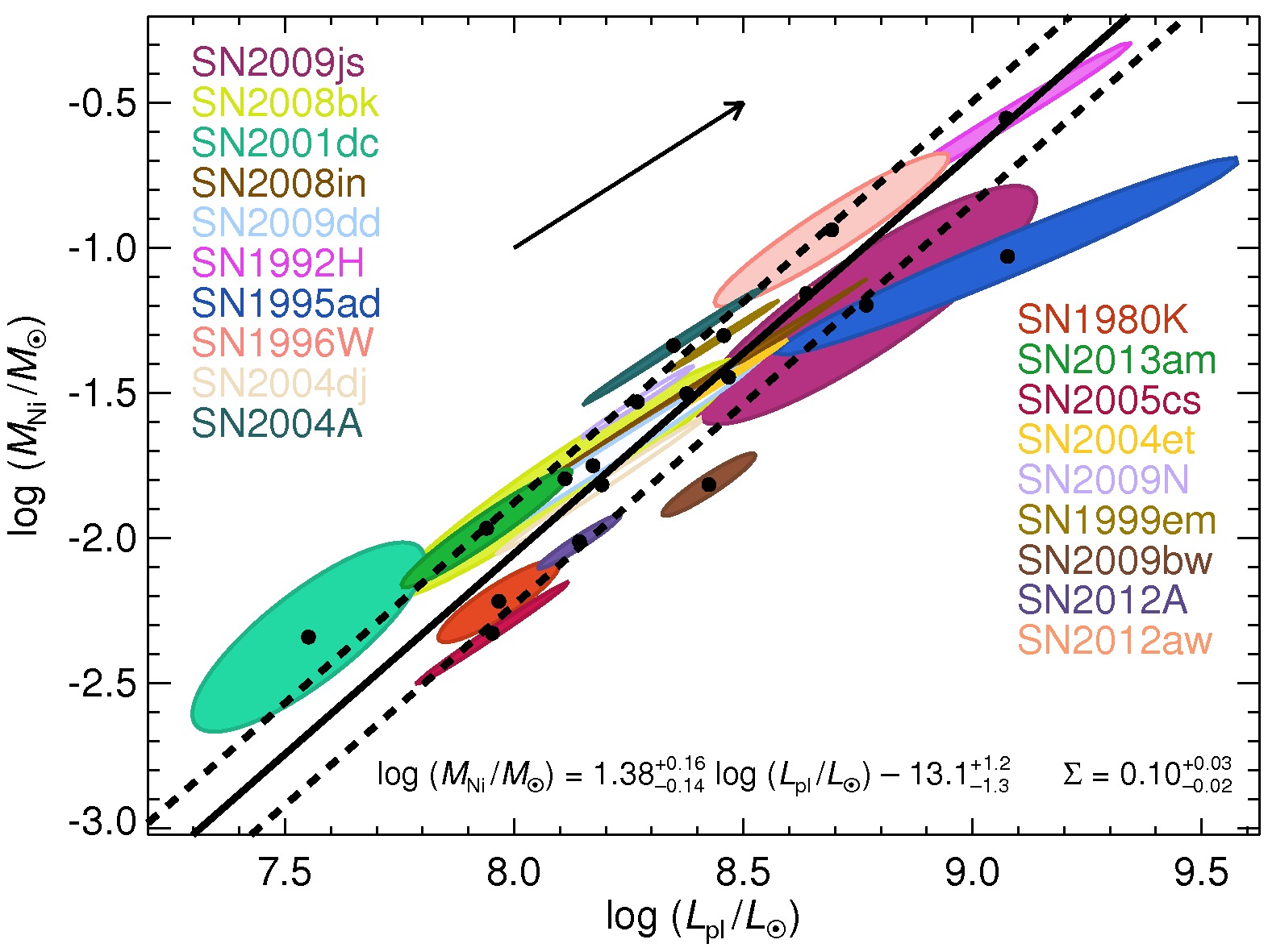
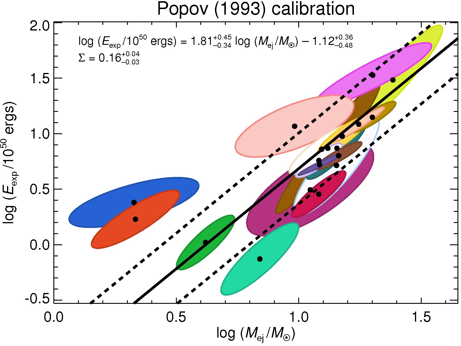
Here we give the plateau luminosities, nickel masses, explosion energies, and progenitor radii obtained using scaling relations from light curves fitted with the method of Pejcha & Prieto (2015, ApJ, 799, 215).
Litvinova & Nadezhin (1985) calibration of the scaling relations
Popov (1993) calibration of the scaling relations
Identification of supernova names
The column structure of the first two files is:
Sample IDL code to plot confidence ellipsoids like in our paper. covar is an array of covariance matrix coefficients obtained by reading the files above:
plot1 = 2   ; variables to plot, here M_Ni vs E_exp
plot2 = 0

cov = reform(covar, 5,5)
my_cov[0,0] = cov[plot1,plot1]
my_cov[0,1] = cov[plot1,plot2]
my_cov[1,0] = cov[plot2,plot1]
my_cov[1,1] = cov[plot2,plot2]

invc = invert(my_cov,/double)
r2 = 2.30/(invc[0,0]*cp^2 + 2.0*invc[0,1]*cp*sp + invc[1,1]*sp^2)	;; factor 2.30 is related to number of variables and confidence level and is explained in Numerical Recipes
r = sqrt(r2)
x = r*cp	;; these are x and y coordinates of the 1-sigma confidence elipsoid relative to the datapoint
y = r*sp